1. Van der Pol

The Van der Pol equation is a second-order nonlinear ordinary differential equation used to model oscillatory systems with damping. It is expressed as:

(1)\[\begin{equation} \frac{d^2x}{dt^2} = \mu(1 - x^2)\frac{dx}{dt} - x. \end{equation}\]

where \(x\) denotes the position coordinate. Its first derivative represents velocity, and its second derivative represents acceleration. The parameter \(\mu\) controls the nonlinearity and damping strength. For small values of \(\mu\), the system exhibits stable oscillations, while larger values of \(\mu\) lead to more pronounced nonlinear behavior. The Van der Pol equation is often used to study nonlinear dynamics and serves as a classic example of self-sustained oscillations [1].

In this tutorial, we use the Van der Pol equation as a straightforward example to demonstrate the CVODE solver. We choose a large value of \(\mu\) to make the system stiff, and we match all input parameters and times to those in a similar example from MATLAB for ease of comparison.

1.1. Problem setup

Although the problem is a second-order ODE, most solvers are designed to be more efficient with first-order ODEs. Therefore, we will convert the problem to first-order derivatives by letting \(y = [x, \dot{x}]\). Taking the derivative of \(y\) gives \(\dot{y} = [\dot{x}, \ddot{x}]\). This results in a system of two first-order ODEs, which can be written as:

(2)\[\begin{align} \dot{y}_0 &= \dot{x} = y_1, \\ \dot{y}_1 &= \ddot{x} = \mu(1 - x^2)\frac{dx}{dt} - x = \mu(1 - y_0^2)y_1 - y_0. \end{align}\]

Notice how substitutions are used throughout the expressions to write the problem entirely in terms of \(y\) rather than \(x\). Once a problem is in a first-order form it can easily be translated into a Python function that the CVODE solver can interpret.

The CVODE solver is accessed by creating an instance of the sundae.cvode.CVODE class. The only required input is a right-hand-side function (rhsfn) that defines the \(\dot{y}\) array of derivatives. Rather than a return value, rhsfn must have a signature like f(t, y, yp) where yp is a pre-allocated array that can be filled within the function. For more details, refer to the documentation. Below, the rhsfn function is set up to match the expressions above, with \(\mu=1000\).

import numpy as np
import numpy.testing as npt

import sksundae as sun
import matplotlib.pyplot as plt

def rhsfn(t, y, yp):
    yp[0] = y[1]
    yp[1] = 1000*(1 - y[0]**2)*y[1] - y[0]

1.2. Solve and plot

Now that rhsfn is defined, it can be used to create an instance of CVODE. We will use all default options here, but note that many options for tolerance, constraints, and other parameters can be set during class initialization.

Once the solver is constructed, it can be run using one of two methods: step or solve. The solve method integrates over a defined time span while the step method performs one integration step at at time. First, we’ll demonstrate how to use the solve method, which requires the integration time span and an initial condition y0 (i.e., the values of \(y\) at tspan[0]).

The solver detects how the solution should be recorded in time based on the length of tspan. When given exactly two values, as in the example below, the solver returns the solution at internally chosen time steps between the two values. When it is important to evaluate the solution at specific times, tspan should be an array with length greater than 2, specifying the times at which the solution should be recorded for output.

tspan = np.array([0, 3000])
y0 = np.array([2, 0])

solver = sun.cvode.CVODE(rhsfn)
soln = solver.solve(tspan, y0)
print(soln)

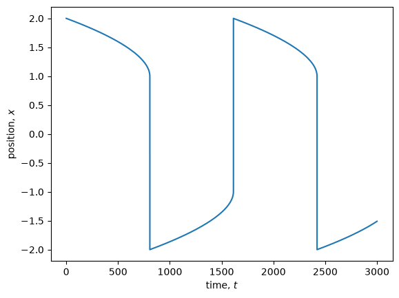
plt.plot(soln.t, soln.y[:,0])
plt.xlabel("time, $t$");
plt.ylabel("position, $x$");

  message: Reached specified tstop.
  success: True
   status: 1
        t: [ 0.000e+00  2.686e-08 ...  2.970e+03  3.000e+03]
        y: [[ 2.000e+00  0.000e+00]
            [ 2.000e+00 -5.371e-08]
            ...
            [-1.544e+00  1.114e-03]
            [-1.510e+00  1.178e-03]]
 i_events: None
 t_events: None
 y_events: None
     nfev: 1905
     njev: 31

1.3. Step-wise solutions

Solving step-by-step instead of across a full time span can be beneficial in some cases, especially for debugging. Therefore, a step method is also available in CVODE. Before taking a step, the solver needs to know the initial conditions and time to determine the direction of integration for the following steps. Thus, before calling step, you should call init_step, as shown below. The initialization is handled automatically when using the solve method but must be done manually in a step-by-step approach.

Below, we run init_step and compare the solution soln_0 to the initial values from the full solve, from above. Afterward, we take a step evaluated at soln.t[10] using the solution object from the full solve, allowing us to compare the step-by-step solution to a portion of the full solution. We only check that the solutions are within some tolerance (1e-7) because the solver’s internal steps may differ from those in the full solution, meaning the values will be close but may not be exactly the same.

soln_0 = solver.init_step(0, y0)
print(soln_0)

npt.assert_allclose(soln_0.t, soln.t[0])
npt.assert_allclose(soln_0.y, soln.y[0], atol=1e-7)

soln_1 = solver.step(soln.t[10])
print(soln_1)

npt.assert_allclose(soln_1.t, soln.t[10])
npt.assert_allclose(soln_1.y, soln.y[10], atol=1e-7)

  message: Successful function return.
  success: True
   status: 0
        t: 0.0
        y: [ 2.000e+00  0.000e+00]
 i_events: None
 t_events: None
 y_events: None
     nfev: 0
     njev: 0


  message: Successful function return.
  success: True
   status: 0
        t: 0.0005614010396975667
        y: [ 2.000e+00 -5.451e-04]
 i_events: None
 t_events: None
 y_events: None
     nfev: 20
     njev: 1

The step method also has optional settings that you should explore and review in the full documentation. Notably, there is a method keyword argument that controls how the step is taken. The normal method will integrate all the way to the specified t value. Alternatively, you can use the onestep method which will allow the solver to take one internal time step toward t. This can result in the output value being somewhere between the previous time and the current t value, or may also result in the solver taking a step past the “requested” t. If you want to guarantee the solver does not step past a given time, use the tstop option. You can read more about tstop in the full documentation.

Although it might be tempting to use the step method to mix taking steps both forward and backward in time, relative to a previous step, the solver is designed to integrate in a single direction. Therefore, each time step should be chosen carefully (or tstop should be set for each step) to avoid stepping past a value that you cannot return to.

1.4. Advanced features

The CVODE solver offers many advanced settings and controls. While we won’t cover all of them in detail, we will discuss two important ones: (1) event functions and (2) Jacobian functions.

1.4.1. Event functions

Event functions allow the solver to record solutions based on some criteria of interest, and if requested, can also terminate the solution when the criteria occurs. As a basic example, imagine throwing a ball straight up in the air and tracking its vertical position. You may want to record the time and location in which the ball reaches a maximum height, and also may want to force the solver the quit when the ball hits the ground so that you do not end up with unphysical solutions (i.e., the ball had negative height). To allow the solver to track events, you need to define a function with a signature like f(t, y, events). Inside the function, the events array should be filled with expressions that define an event. An event is triggered if any events[i] = 0 during the solve. The solver needs to know two things when using events: (1) the events function itself, passed using the eventsfn keyword argument, and (2) the number of events to track, passed using num_events. Below we set up two events that track when y[0] is equal to 1 and when y[1] = yp[0] = 0 (i.e., when the oscillator changes direction).

After being defined, you may also decide to change the optional terminal and direction attributes for your events function. These attributes dictate what happens when an event occurs. Each attribute must be a list with the same number of values as num_events, allowing each event to have its own terminal and direction behavior. terminal values can be True or False to specify that the solver should or should not stop integrating when the specified event occurs, respectfully. You can also set an integer terminal value to tell the solver that it should only exit after the corresponding event has occurred some number of times. direction specifies when an event should be ignored based on the sign change of an events[i] expression. In the example below, the terminal and direction values are set to do the following:

• Tell the solver to stop only after y[0] = 1 has occurred three times.

• Record the solution when y[1] = 0, but do not stop integration if this occurs.

• Regardless of which direction y[0] = 1 happens (i.e., when events[0] has either positive or negative slope), record this event and include it toward the terminal count.

• The y[1] = 0 event should only be recorded if events[1] has a positive slope when it is detected. Therefore, y[1] = yp[0] went from being negative to positive (a local minima). Although y[1] = yp[0] = 0 may also represent a local maxima, these are ignored here.

def eventsfn(t, y, events):
    events[0] = y[0] - 1
    events[1] = y[1]
    
eventsfn.terminal = [3, False]
eventsfn.direction = [0, 1]
    
solver = sun.cvode.CVODE(rhsfn, eventsfn=eventsfn, num_events=2)
soln = solver.solve(tspan, y0)
print(soln)

plt.plot(soln.t, soln.y[:,0], '-', soln.t_events, soln.y_events[:,0], 'or')
plt.xlabel("time, $t$");
plt.ylabel("position, $x$");

  message: Detected one or more events.
  success: True
   status: 2
        t: [ 0.000e+00  2.686e-08 ...  2.421e+03  2.421e+03]
        y: [[ 2.000e+00  0.000e+00]
            [ 2.000e+00 -5.371e-08]
            ...
            [ 1.001e+00 -9.669e-02]
            [ 1.000e+00 -1.021e-01]]
 i_events: [[-1  0]
            [ 0  1]
            [ 1  0]
            [-1  0]]
 t_events: [ 8.068e+02  8.069e+02  1.614e+03  2.421e+03]
 y_events: [[ 1.000e+00 -1.021e-01]
            [-2.000e+00  2.475e-11]
            [ 1.000e+00  1.334e+03]
            [ 1.000e+00 -1.021e-01]]
     nfev: 1478
     njev: 25

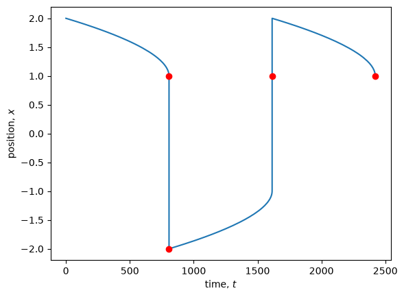
The solution output demonstrates that the events were tracked correctly. All specified events were tracked and recorded according to the specified settings. In addition to the t_events and y_events values in the solution object, which are self explanatory, the i_events field gives you information on which event triggered each record and which direction the event was detected going when it was recorded. For example, the first row means that the events[0] expression was detected with negative slope.

There are a couple more things you should be aware of if you decide to use events. First, if you don’t specify terminal or direction, the default behavior is to make all events terminate integration on their first occurrence and to track both positive and negative slopes for each events[i]. Lastly, when an event is terminal, the results for that event occurrence are output to both the main arrays (t and y) and then “events” arrays (t_events and y_events) within the solution object. In contrast, if an event is not terminal, it is only recoded in the “events” arrays.

1.4.2. Jacobian functions

In this simple and small problem, the solver is already fast and requires minimal computational effort. However, for larger problems, you can benefit from explicitly defining the Jacobian of your system. When the Jacobian is not provided, the solver numerically approximates it by perturbing the state variables \(y\). For large systems of equations, this numerical approximation can be time-consuming, especially if performed frequently, which may significantly slow down the integrator. In such a case, you may benefit from defining the Jacobian function yourself. The Jacobian is defined as

(3)\[\begin{equation} J_{ij} = \frac{df_i}{dy_j}, \end{equation}\]

where \(f_i\) are the right-hand-side expressions from rhsfn and \(y_j\) are the variables in the \(y\) array. Note that the Jacobian is a 2D array where each row corresponds to an \(f\) expression and each column is associated with a specific \(y\). The Jacobian function must have a signature like J(t, y, yp, JJ) where JJ is a pre-allocated 2D array that should be filled within the function. yp are the values of the rhsfn at the current time. The Jacobian function for the Van der Pol problem is given below and is passed to the solver using the jacfn keyword argument.

def jacfn(t, y, yp, JJ):
    JJ[0,0] = 0
    JJ[0,1] = 1
    JJ[1,0] = -2000*y[0]*y[1] - 1
    JJ[1,1] = 1000*(1 - y[0]**2)
    
solver = sun.cvode.CVODE(rhsfn, jacfn=jacfn)
soln = solver.solve(tspan, y0)
print(soln)

plt.plot(soln.t, soln.y[:,0])
plt.xlabel("time, $t$");
plt.ylabel("position, $x$");

  message: Reached specified tstop.
  success: True
   status: 1
        t: [ 0.000e+00  2.686e-08 ...  2.977e+03  3.000e+03]
        y: [[ 2.000e+00  0.000e+00]
            [ 2.000e+00 -5.371e-08]
            ...
            [-1.537e+00  1.128e-03]
            [-1.510e+00  1.180e-03]]
 i_events: None
 t_events: None
 y_events: None
     nfev: 1963
     njev: 32

You should consider providing the Jacobian for your problem when the number of Jacobian evaluations (njev) is large or when the problem size is substantial and the solver is slow to return results.

In some cases, you may also be able to speed up the solver without explicitly providing the Jacobian. If your problem has a banded Jacobian, you can switch to the banded solver using the option linsolver='band' when initializing your class. You will also need to specify the lower and upper bandwidths using the lband and uband options. This approach avoids the need to explicitly write out the Jacobian. The numerical algorithm for approximating banded Jacobians is significantly more efficient than the default dense method for problems having sparse Jacobians with narrow bandwidths. However, if the bandwidth is large, it may still be beneficial to explicitly provide jacfn. Both dense and band linear solvers support the jacfn option, but the band option will generally be faster if your bandwidth is less than the full matrix dimensions.