Linear Solvers#
SUNDIALS (Suite of Nonlinear and Differential/Algebraic Equation Solvers) provides efficient linear solvers tailored for solving systems of equations arising in scientific computing. The two primary types of linear solvers available in SUNDIALS are band and dense solvers. These solvers cater to different problem structures, optimizing performance and computational efficiency.
Dense Solvers#
Dense solvers are suitable for systems where the Jacobian matrix is fully populated with non-zero entries. While they can handle banded problems, they may be less efficient than banded solvers in cases where sparsity exists.
When to Use:
Opt for a dense solver when the Jacobian matrix does not exhibit a banded structure.
Ideal for smaller systems where the overhead of manipulating the problem into a banded structure may outweigh the benefits.
Banded Solvers#
Banded solvers are designed for systems where the Jacobian matrix is sparse and has non-zero entries concentrated around the diagonal. This structure is common in problems derived from finite difference methods or certain discretizations of partial differential equations.
When to Use:
Use a band solver when the Jacobian matrix has a banded structure.
Beneficial for large systems. When possible, try to order your problem’s systems of equations to minimize the bandwidth.
Configuration in scikit-SUNDAE#
Switching between SUNDIALS linear solvers in scikit-SUNDAE is straightforward. While initializing your solver, simply specify which linear solver to use. The dense linear solver is the default. Changing to a banded linear solver is the same in both the CVODE and IDA solvers as demonstrated below:
from sksundae.ida import IDA
from sksundae.cvode import CVODE

# IDA with a dummy residuals function
def resfn(t, y, yp, res):
    pass

L = 0  # lower bandwidth
U = 0  # upper bandwidth

solver = IDA(resfn, linsolver='band', lband=L, uband=U)

# COVDE with a dummy right-hand-side function
def rhsfn(t, y, yp):
    pass

L = 0  # lower bandwidth
U = 0  # upper bandwidth
solver = CVODE(rhsfn, linsolver='band', lband=L, uband=U)
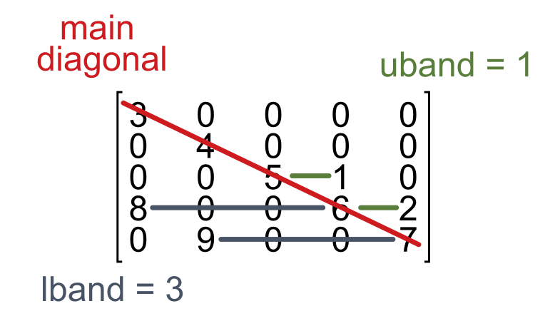
Ensure you provide both the lower bandwidth lband and upper bandwidth uband when using the band linear solver. Each bandwidth defines the LARGEST distance between a non-zero element and the main diagonal, on either side, as shown in the figure below. Forgetting to set either bandwidth will raise an error. If lband + uband matches the dimension N of the matrix, the performance of the band and dense linear solvers will be approximately the same.
In the limiting case where the Jacobian is only non-zero along the main diagonal, both bandwidths can be zero. However, it is unlikely that you will be able to find many, if any, problems that fit this exact form.
Performance Considerations#
Choosing between band and dense solvers depends primarily on the structure of your Jacobian matrix. Banded solvers can significantly reduce memory usage and improve computational speed for large systems with banded matrices, while dense solvers may be more straightforward for smaller, fully populated matrices.
In either case, the default algorithm will numerically approximate the Jacobian for you. However, there are fewer elements for the solver to calculate when using band since it focusses on a subset of the Jacobian matrix, around the diagonal. You can further improve the performance of either solver by explicitly providing the Jacobian, as we cover here.
Further Reading#
For more detailed information on the linear solvers and their implementation, please refer to the SUNDIALS documentation. However, be aware that their full documentation covers more solvers than are implemented in scikit-SUNDAE.